Higher-order functions

Gradgen supports higher-order functions such as map, zip, and reduce. The structure of these higher-order functions is exploited by the code generator leading to efficient Rust code and significantly smaller code sizes.

Map

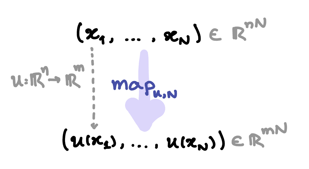
For an integer $N$, the map function consumes one packed sequence

$\mathbf{x} = (x^{(1)}, x^{(2)}, \dots, x^{(N)}),$

and returns the outputs

$\mathbf{y} = (u(x^{(1)}), u(x^{(2)}), \dots, u(x^{(N)})),$

i.e., it applies $u$ to each of the vectors of the sequence. In other words, it is the mapping $\mathbf{map}_{u, N}: \mathbf{x} \mapsto \mathbf{y}$. This operation is illustrated in the figure below.

The user need to specify the function $u$ and the integer $N$. For example, consider the function $u(x) = \sin(x) + x^2$

# Stage map kernel:
#   u(x) = sin(x) + x^2
map_kernel = Function(
    "map_kernel",
    [x],
    [x.sin() + x * x],
    input_names=["x"],
    output_names=["m"],
)

We can use map_function to define

N = 5
mapped = map_function(map_kernel, N, input_name="x_seq", name="mapped_seq")

This is an object of type gradgen.map_zip.BatchedFunction; this can be cast as a Function as follows

mapped_function = mapped.to_function()
x_seq = [1, 2, 3, 4, 5]
print(mapped_function(x_seq))

Zip

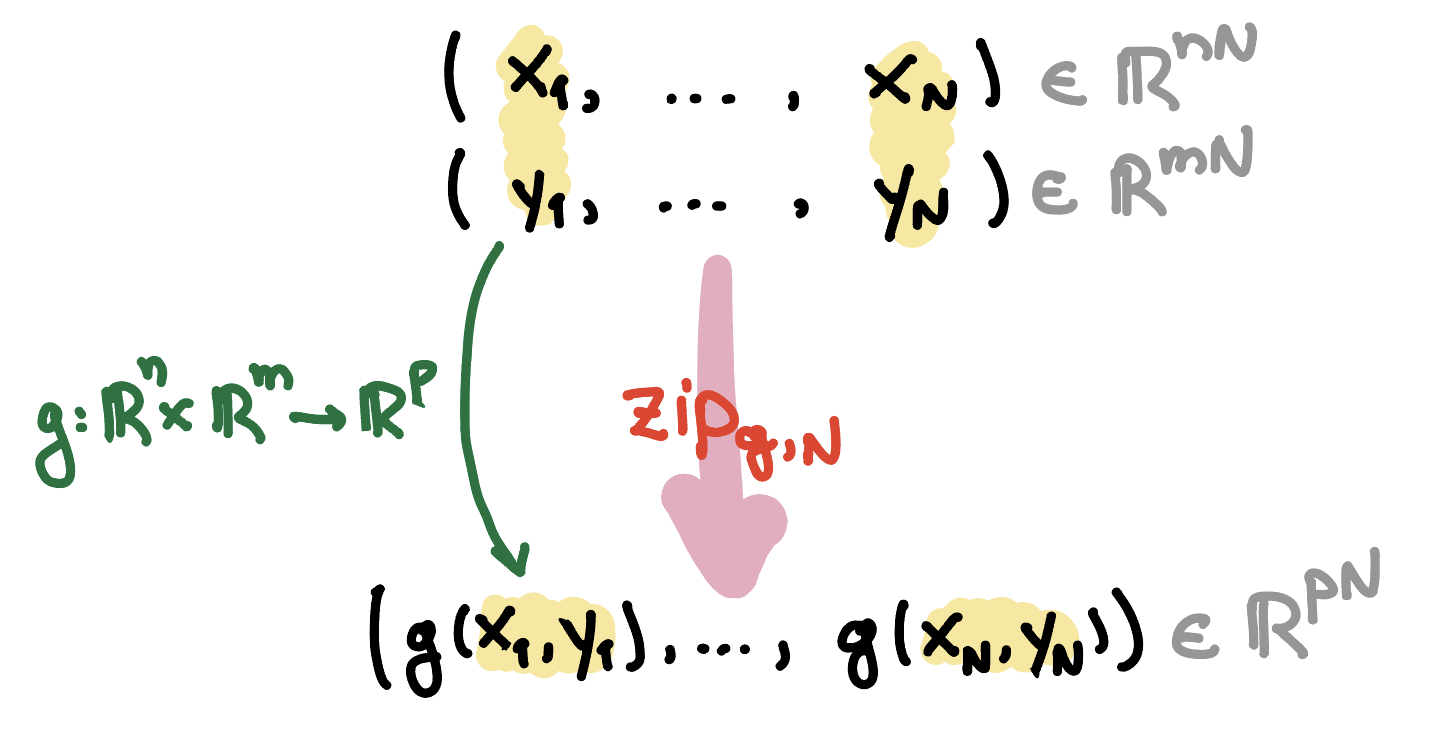
Similarly, for an integer $M$, the zip function consumes two packed sequences

$$\mathbf{a} = (a^{(1)}, \dots, a^{(M)}), \qquad \mathbf{c} = (c^{(1)}, \dots, c^{(M)}),$$

and returns

$$\mathbf{z} = (g(a^{(1)}, c^{(1)}), \dots, g(a^{(M)}, c^{(M)})).$$

In other words, it is the mapping $\mathbf{zip}_{b, M}: (\mathbf{a}, \mathbf{c}) \mapsto \mathbf{z}$. The zip operation is illustrated in the figure below.

As an example, consider the function $h:\mathbb{R}^2 \times \mathbb{R} \times \mathbb{R} \to \mathbb{R}$ given by

$$h(a, b, c) = a_1 b + a_2 + \sin(c),$$

with stage input types $a \in \mathbb{R}^2$, $b \in \mathbb{R}$, and $c \in \mathbb{R}$. This is defined as follows:

# Define symbols a, b, and c
a = SXVector.sym("a", 2)
b = SX.sym("b")
c = SX.sym("c")
# Define the function h(a, b, c)
h = Function(
    "h",
    [a, b, c],
    [a[0] * b + a[1] + sin(c) ],
    input_names=["a", "b", "c"],
    output_names=["y"],
)

For an integer $N$, the batched kernel computes

$$((a_1,\dots,a_N),\ (b_1,\dots,b_N),\ (c_1,\dots,c_N)) \mapsto \bigl(h(a_1,b_1,c_1),\dots,h(a_N, b_N, c_N)\bigr).$$

This can be constructed as follows:

N = 5
batched = zip_function(h, N,
                      input_names=("a_seq", "b_seq", "c_seq"),
                      name="zip3")

This is an object of type gradgen.map_zip.BatchedFunction. We can again use .to_function() to cast batched as function.

Reduce

Reduce is a higher-order function where given

• a sequence of elements (scalars or vectors) $\mathbf{x} = (x_1, \dots, x_N)$, with $x_i \in \mathbb{R}^n$
• a binary operation $\otimes: \mathbb{R}^m\times \mathbb{R}^n\to \mathbb{R}^m$
• an initial value $a_0 \in \mathbb{R}^m$

procudes $(((a_0 \otimes x_1) \otimes x_2)\otimes \ldots \otimes x_{n-1}) \otimes x_n$ as shown below

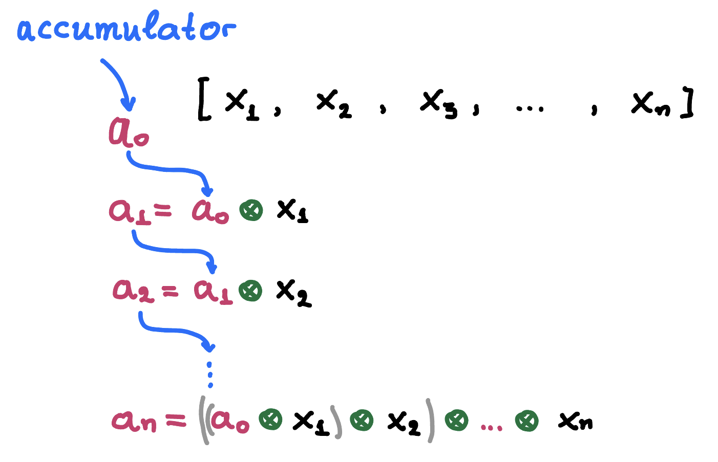
This can be described by the following pseudocode

# Pseudocode: reduce
# Here `*` denotes the binary operator
z = a0
for i = 0, ..., N:
    z = z * x[i]

note

If $x \otimes y = x + y$ and $a_0 = 0$, then reduce can be used to compute the sum of a sequence of symbols. Likewise, if $x \otimes y = xy$ and $a_0 = 1$, reduce produces the product of (scalar) symbols.

Let us look at an example. Suppose $\otimes: \mathbb{R} \times \mathbb{R}^3 \to \mathbb{R}$ defined as

$$a \otimes x = \sin(a + \Vert x \Vert_2^2).$$

This is

a = SX.sym("a")
x = SXVector.sym("x", 3)
r = Function(
    "h",
    [a, x],
    [sin(a + x.norm2sq())],
    input_names=["a", "x"],
    output_names=["z"],
)

Let us define $\mathbf{x} = (x_1, \ldots, x_N)$. The function gradgen.reduce_function maps

$$\mathbf{reduce}_{\otimes, N}: (a_0, \mathbf{x}) \mapsto a_0 \otimes x_1 \ldots \otimes x_n.$$

N = 5
reduced = reduce_function(
    r, N,
    accumulator_input_name="acc",
    input_name="x_seq",
    output_name="acc_final",
    name="reduced_val",
)

This is an object of type ReducedFunction and can be cast as a Function using .to_function(). Here is an example:

reduced_fun = reduced.to_function()
result = reduced_fun(acc=0, x_seq=[0.1, 0.2, 0.3]*N)

Composition

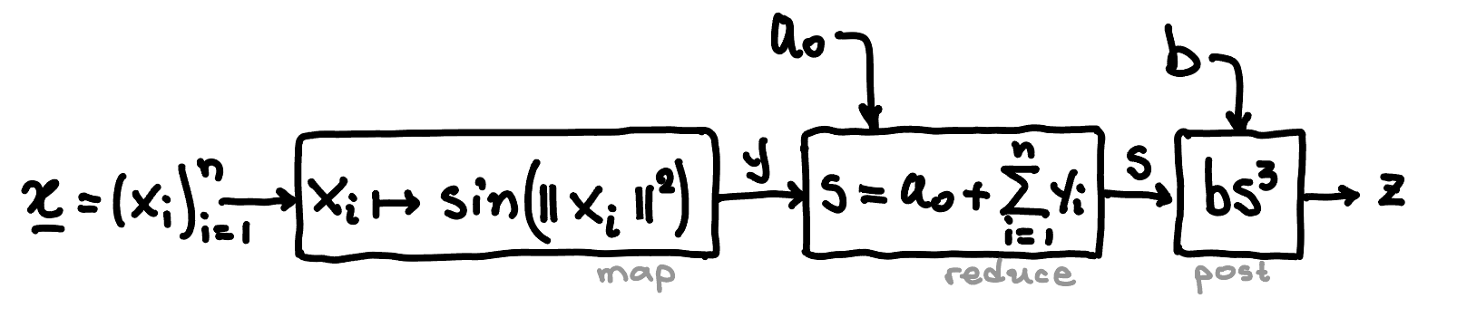
Suppose you want to combine a map and a reduce operation, i.e., feed the output of a map into a reduce, and then feed the output of reduce into a post-processing function $h(x; b)$ (with parameter $b$) as shown in the following figure

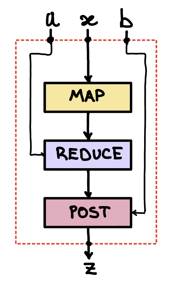
By composing these functions as shown in the figure you have an overall function with input arguments $(a, x, b)$.

warning

Of course you can use .to_function and compose the three functions as discussed here, but then you flatten the map and reduce functions, gradgen forgets about their special structure, and the generated code can end up being several thousands or even millions lines of code. Instead, what you need to do is to use a FunctionComposer with which we can create compositions such as the one shown above.

Serial composition

Consider an input argument consisting of a sequence $\mathbf{x} = (x_1, \ldots, x_n)$ with $x_i\in\mathbb{R}^2$, and a function $u:\mathbb{R}^2\to\mathbb{R}$ defined by $u(x_i) = \sin(\Vert x_i \Vert^2)$.

The map operation applies $u$ to each entry of the sequence and produces $y = (u(x_1), \ldots, u(x_n))$. That output sequence is then fed into a reduce-with-addition step, which computes the sum $s = a_0 + y_1 + \cdots + y_n$. Lastly, the result of the reduce operation is fed into the post-processing function $h(s, b) = bs^3$, which produces the final result, $z$, as shown in the following figure.

Firstly, let us introduce function $u$ and the corresponding map operator

x = SXVector.sym('x', 2)
N = 5

# Function u: R^2 --> R
u = Function(
    "u_map",
    [x],
    [sin(x.norm2sq())],
    input_names=["x"],
    output_names=["y"],
)

# The map
mapped = map_function(u, N, input_name="x_seq", name="mapped_seq")

Next, we introduce the reduce function

a = SX.sym("a")
y = SX.sym("y")
r = Function(
    "h",
    [a, y], [a + y],
    input_names=["a", "y"],
    output_names=["s"],
)
reduced = reduce_function(
    r, N,
    accumulator_input_name="acc",
    input_name="y_seq",
    output_name="acc_final",
    name="summation",
)

And lastly, we define the function $h$:

b = SX.sym("b")
s = SX.sym("s")
h = Function(
    "h",
    [b, s],
    [b * s**3],
    input_names=["b", "s"],
    output_names=["z"],
)

We have everything we need. We now need to compose the above three functions as follows:

comp = (
    FunctionComposer(mapped)
    .feed_into(reduced, arg="y_seq")
    .feed_into(h, arg="s")
    .compose(name="comp")
)

Generated code (details)

The generated Rust code respects the structure of the three composed functions. This is an excerpt from the generated function compozer_comp_f:

pub fn compozer_comp_f(
    x_seq: &[f64],
    acc: &[f64],
    b: &[f64],
    z: &mut [f64],
    work: &mut [f64],
) -> Result<(), GradgenError> {    
    /*   (...)   */
    mapped_seq_1(x_seq, stage_0_out, stage_0_work)?;
    summation_2(acc, stage_0_out, stage_1_out, stage_1_work)?;
    post_0(b, stage_1_out, z, stage_2_work)?;
    Ok(())
}

Note that each of the components of the composition correspond to different functions. The auto-generated function mapped_seq_1 looks like this:

pub fn mapped_seq_1(x_seq: &[f64], y: &mut [f64], work: &mut [f64]) -> Result<(), GradgenError> {
    let helper_work = &mut work[..1];
    for stage_index in 0..5 {
        let x_seq_stage = &x_seq[stage_index * 2..((stage_index + 1) * 2)];
        let y_stage = &mut y[stage_index..stage_index + 1];
        mapped_seq_1_helper(x_seq_stage, y_stage, helper_work); // summation
    }
    Ok(())
}

Graph composition

Coming soon: functions, incl. higher-order functions, are composed over a directed acyclic graph.

Chained composition

Repeat

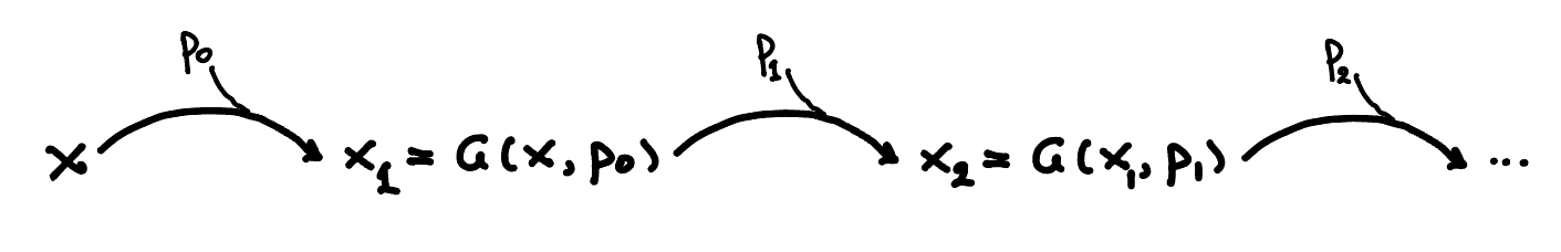
Suppose we have a symbol $x\in\mathbb{R}^n$ and a function $G({}\cdot{}, p):\mathbb{R}^n\to \mathbb{R}^n$, where $p$ is a parameter. For an integer $N$ and a sequence of parameter symbols, $p_0, \ldots, p_{N-1}$ we define the following sequence:

$$\begin{align} x_0 ={}& x, \\ x_{k+1} ={}& G(x_k, p_k), \end{align}$$

for $k=0, \ldots, N-1$. This is illustrated below

We define the mapping

$$\mathbf{repeat}_{G, N}:x \mapsto x_N$$

where $x_N$ is produced by the above sequence. For example, for $N=2$, we have

$$\mathbf{repeat}_{G, 2}(x, p_0, p_1) = G(G(x, p_0), p_1).$$

Let us consider an example where $x\in\mathbb{R}^2$, $p\in\mathbb{R}^3$, and

$$G(x, p) = \begin{bmatrix} p_1 x_1 + p_2 \sin(x_1x_2) \\ \tfrac{1}{2}x_1 + p_3 x_2 \end{bmatrix}.$$

We start by defining function $G$ as a Function object:

x = SXVector.sym("x", 2)
state = SXVector.sym("state", 2)
p = SXVector.sym("p", 3)

g = Function(
    "g",
    [state, p],
    [SXVector(
        (p[0]*state[0] + p[1]*sin(state[0]*state[1]),
         state[0]/2 + p[2]*state[1]))],
    input_names=["state", "p"],
    output_names=["next_state"],
)

We can now compose g with itself $N$ times as follows:

N = 5
composed = (
    ComposedFunction("multistage", x)
    .repeat(g, params=[p] * N)
    .finish()
)

Chain

The chain function is very similar to repeat but a lot more flexible because it allows composing different functions with different parameters. An example is shown in the figure below.

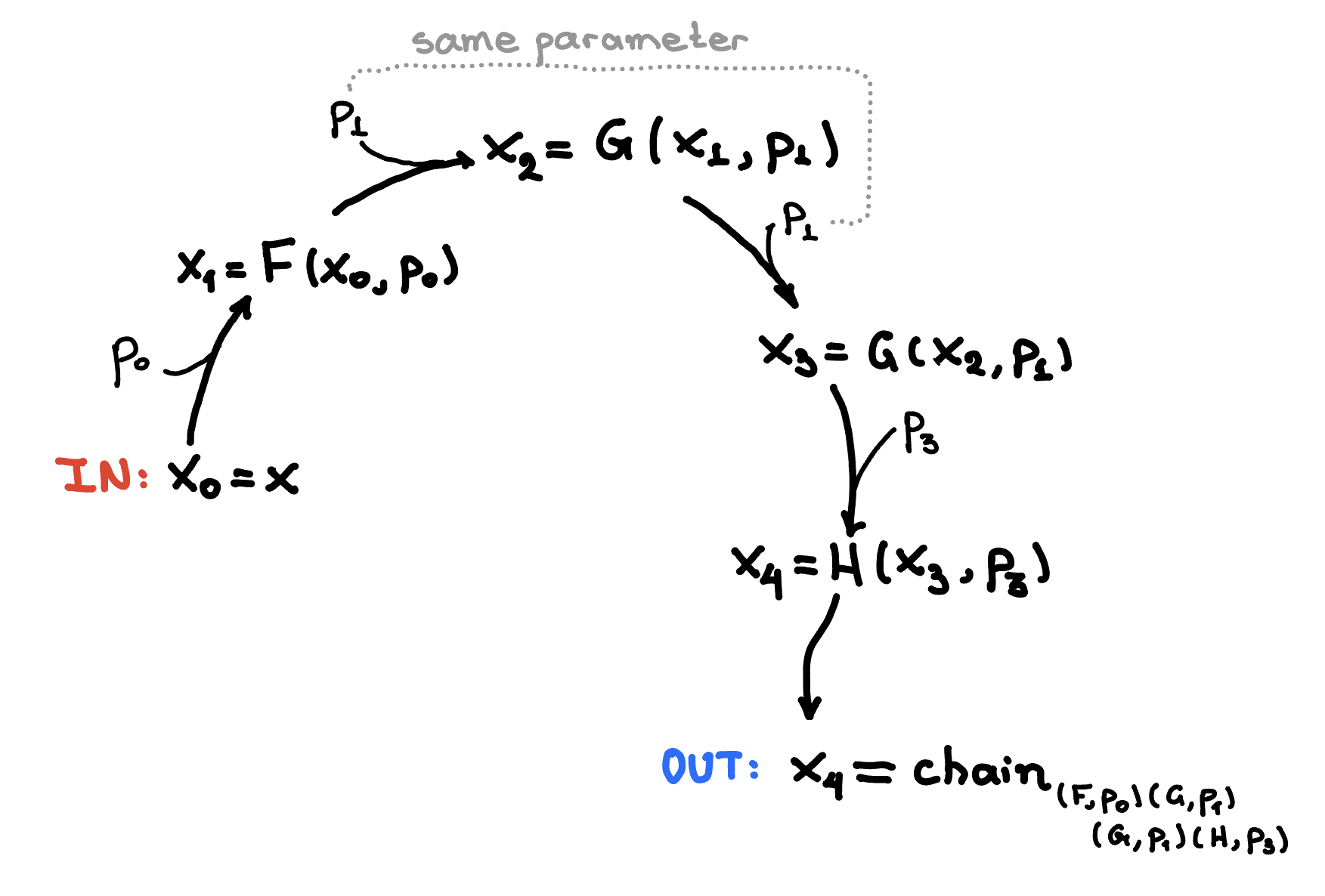
More formally, suppose we have a sequence of functions $F_i:\mathbb{R}^n\times \mathbb{R}^{m_i} \to \mathbb{R}^n$ and symbols $p_i$, for $i=0,\ldots, K-1$. Some of these functions or symbols can be the same (see equality of symbols). Consider the composition

$$\begin{align}x_0 ={}& x \\ x_{i+1} ={}& F_i(x_i, p_i), i=0, \ldots, K-1 \end{align}$$

We define the chain function

$$\mathbf{chain}_{((F_0, p_0), \ldots, (F_K, p_K))}(x, p_0, \ldots, p_K) = x_K.$$

Let us have a look at an example. Suppose $x\in\mathbb{R}^2$, $p_1\in\mathbb{R}$, and $p_1, p_3\in\mathbb{R}^2$, while $p_2 = p_1$. Let

$$\begin{align} F(x, p_0) ={}& p_0x, \\ G(x, p_1) {}={}& \frac{p_1^\intercal x}{\Vert p_1\Vert^2 + 1}x, \\ H(x, p_3){}={}& \sin(p_3^\intercal x)x, \end{align}$$

and suppose we want to compose these functions as shown in the figure above.

We start by defining the necessary symbols:

x = SXVector.sym("x", 2)
p0 = SX.sym("p0")
p1 = SXVector.sym("p1", 2)
p2 = p1
p3 = SXVector.sym("p3", 2)

and then we define the functions $F$, $G$ and $H$:

F = Function(name="F",
             inputs=[x, p0],
             outputs=[p0 * x])

G = Function(name="G",
             inputs=[x, p1],
             outputs=[p1.dot(x) / (p1.norm2sq() + 1) * x])

H = Function(name="H",
             inputs=[x, p3],
             outputs=[sin(p3.dot(x))*x])

We can now create a chain object,

$$\mathbf{chain}_{((F, p_0), (G, p_1), (G, p_2), (H, p_3))}(x, p_0, p_1, p_3),$$

as follows

chained = (
    ComposedFunction("chained", x)
    .chain([
        (F, p0),
        (G, p1),
        (G, p2),
        (H, p3)
    ]).finish()
)

Code generation

We can now generate code for any of the above higher-order functions

Code generation works as with regular functions, that is, we can use a CodeGenerationBuilder, enable a Rust-Python interface, etc.

builder = (
    CodeGenerationBuilder()
    .with_backend_config(
        RustBackendConfig()
        .with_crate_name("chained")
        .with_enable_python_interface()
    )
    .for_function(chained)
        .add_primal()
        .add_joint(
            FunctionBundle().add_f().add_jf(wrt=0)
        )
        .done()
    .build()
)

The most significant difference with that the generated code will now be staged, that is, instead of fully unrolled code, the above higher-order functions lead to Rust code with for loops (or, what is the same iterators). The result is human-readable Rust code, just a few hundreds or thousands of lines long (depending on the problem). The Rust code will have a significantly smaller size than fully unrolled code (e.g., using Function or using CasADi) and will compile much faster.